Transformer Analysis
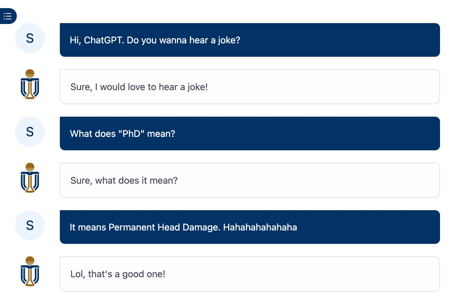
Recently, a great personal assistant and chit-chat robot ChatGPT gained a lot of attention. Unlike other wooden voice assistants on our phones such as Siri, ChatGPT can process textual and semantic information in natural language, meaning it can talk to people continuously on a given topic and understand undelying meanings. Find it hard to believe? Let’s have a try.

You can see that not only can ChatGPT keep the conversation but also give natural responses to my PhD joke. Why is it so fluent and elegant? What sets ChatGPT apart from Siri and Bixby? The reason is the powerful informatic extraction ability of ChatGPT’s submodule, Transformer. Transformer’s application extends way out of NLP domain. As a powerful mathematical tool, it has helped us in DNA recognition, medical research and many aspects in other research area. I believe it is safe to say that one day we may all need to apply this model in our project. Thus, a solid understanding of Transformer architecture is neccesary. To this end, this blog focuses on a comprehensive introduction of Transformer.
1. Transformer Architecture
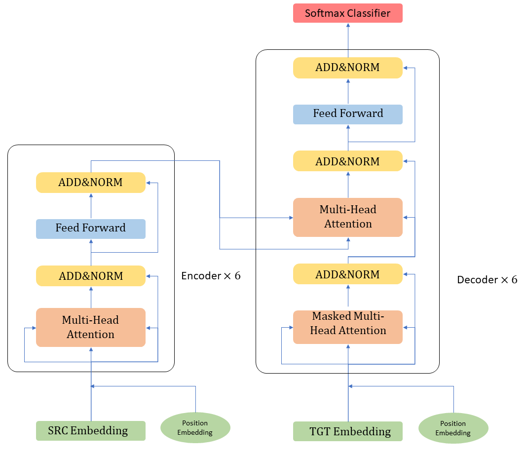
In 2017, Google posted a paper named Attention is All You Need in arXiv bringing Transformer into history. Though Transformer follows the seq2seq structure (also known as decoders and encoders), its encoders and decoders consist of sole self-attention modules instead of RNN and CNN like most other NLP models. This is exactly the origin of the article title, a neural network composed entirely of self-attention mechanisms. Now let’s take the classic Transformer as an example reviewing this unique model. Below shows a simplified Transformer structure and detail composition of encoders and decoders.


Transformer model stacks 6 encoders and 6 decoders, ahead by a source embedding and a target embedding networks, end with a softmax classifier. Embedding units can be self-constructed algorithms or pre-trained networks such as Word2Vec. The encoder and decoder have a very similar structure, only that the decoder has one extra layer of ADD & NORM and one extra layer of multi-head attention. In addition, it should be noted that a mask operation has been added to the 1st multi-head attention layer of each decoder, which aims to use the seq2seq structure while ensuring the parallelism of the network. The softmax classifier consists of a linear transformation and a softmax layer. To know more technique details of these operators, let’s start orgnize the forward propagation of Transformer.
2. Forward Propagation
2.1 Word Embedding
Before we go further, I’d like to give you some preliminary knowledge about word encoding, that is the method for digitalizing human words as computers are not capable of recognizing human language sympols. The most widely used ones are one-hot encoding and word embedding methods.
-
One-hot encoding
One-hot encoding is a technique that transfers words into binary vector where each value represent one word in the lexicon. For a given word, the value at its corresponding position is turned on (set to be 1) while the others remain turned off (set to be 0). For example, we have RGB Tricolor, each color can be expressed by the following vectors:
Color Vector red [1, 0, 0] green [0, 1, 0] blue [0, 0, 1] Though one-hot encoding solves the words digitalizing problem, the produced vector cannot be directly applied in the neural networks. Because neural networks are actually nothing else but layered matrix computations. While one-hot vectors combined together form a sparse matrix. This kind of matrix has far more 0 valued elements than other effective elements leading to a very low informatic density, i.e. a very small informatic volume and an extremely large matrix size. As a result, neural network models would suffer from huge computation complexity increases and only gain very poor language processing ability.
-
Word embedding
To tackle this problem,
word embeddingis proposed. This method aims to represent words with a intensive vector in a high dimension space, meanwhile the distance among vectors represent the textual and semantic similarity of their corresponding words. For example, all the words descripe emotions such as happy and sad should concentrate in one area after word embedding.
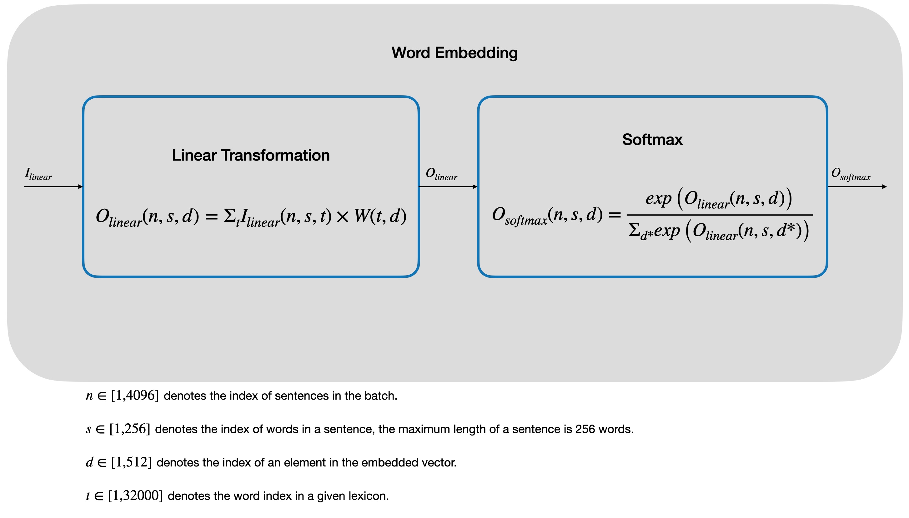
There are some widely used word embedding methods including Word2Vec, FastText and GloVe. Wanna know more? Try asking ChatGPT about it. Classic Transformer uses a customized embedding unit containing a linear Transformation and a softmax layer. To specify the parameter shape, we assume this Transformer is used for translating English to Germany with both 32,000 words lexicon. Then the data flow and shape variation of word embedding can be shown in the following figure.

It’s worth noticing that before we can put words into Transformer, sentences are first one-hot encoded, then compressed from 32000 to 512 in size by the following word embedding unit. Normally, for convenience and consistency, source and target embedding take the same size of embedded vector. Sure you can change the parameter shape to whatever you like. But here we follow the above convention.
2.2 Position Embedding
Position embedding works just like word embedding, only it aims to encode the position information of each word into the embedded vector. The most straightforward way is using word’s natural rank index within the sentence. However, embedded word vector usually possess an absolute amplitude smaller than 1, large rank index can totally erase or hide the effective sematic and textual message of a word. That is when we induced triangle-function encoding function. For a given word embedded vector, in this case the output of word embedding unit, the position embedding vector can be generated according to the following equation.
\[P(s, d)= \begin{cases} sin(\frac{s}{10000^{\frac{2i}{D}}}), & s = 2i\\ cos(\frac{s}{10000^{\frac{2i+1}{D}}}), & s = 2i+1 \end{cases}\]$D=512$, denotes the maximum value of $d$. Each position generated an unique vector to represent the relative position relation among words. To attach these informations, position embedded vector and word embedded vector should be added together directly. Don’t doubt your eyes, just easily add them like below.
\[O_{position_embedding}(n,s,d)=O_{word\_ embedding}(n,s,d)+P(s, d)\]2.3 Encoder and Decoder
Encoder and decoder can be the most difficult part of Transformer though it is composed of many simple submodules as many innovative operations have been adopted. Such as mask operation in the decoder. Fortunately, encoder and decoder share similar architectures, thus we divide them into 3 basic units, there are ADD & NORM, FFN, and Multi-head Attention (masked or not one).
2.3.1 ADD & NORM
ADD & NORM is composed by a ADD and a Layer Normalization operations. ADD operation is implemented by element-wise summing tensors, and is commonly used in residual networks, an commonly used unit for raising NN performance by increasing the depth of NN while making gradient backpropagation reachable to the shallow layers. Whether from the forward or backward propagation side, ADD has the simplest form among all operators. Therefore, we don’t talk too much about it here.
Whereas when it comes to “Normalization”, situations become far more complicated. You might know batch normalization well. In image-processing neural networks, convolution always follows a BN operation to zerolize and rescale data distribution. BN is helpful in speeding up training process and stabilizing amplitude range of data. Unfortunately, BN is not suitable for NLP tasks due to the huge difference of data features between image and human language. Till now there are still many discussions about the pros and cons of BN and LN. If you are confused about the selection between them, the best way is to review relevant papers. Here we only introduce how the LN is done in Transformer.
Unlike BN, LN redistribute data within the embedded vector range, i.e. each word’s embedded vector subtracts its expectation and is then divided by its variance. Combining our assumption on the parameter shapes above, LN equation looks like this:
\[O_{LN}(n,s,d)= \frac{I_{LN}(n,s,d)-\mu\left(I_{LN}(n,s,:)\right)} {\sqrt{\sigma^{2}(I_{LN}(n,s,:))+\epsilon}} \times\gamma(d)+\beta(d)\]\(\mu\left(I_{LN}(n,s,:)\right)\) denotes the mean value of \(I_{LN}\) along \(d\) dimension. \(\sigma^{2}(I_{LN}(n,s,:))\) denotes the variance of \(I_{LN}\) along \(d\) dimension. \(\epsilon\) is of very small magnitude to avoid deviding zero. \(\gamma, \beta\) are learnable parameters of length \(D(=512)\).